Use CMIP6 models together with observational data
Contents
Use CMIP6 models together with observational data#
This example demonstrates how to combine CMIP6 models with observational data from the Copernicus Climate Data Store (CDS). We have chosen Surface Downwelling Longwave Radiation (rlds variable) here. We will load the data, regrid the observational dataset and use it to validate the model. First, load all nesessary libraries.
import intake
import xarray as xr
import cartopy.crs as ccrs
import matplotlib.pyplot as plt
import numpy as np
import xesmf as xe
import cf_xarray as cfxr
import ESMF

%matplotlib inline
print("Using xESMF in version %s" % xe.__version__)
Using xESMF in version 0.6.3
1. Load the model#
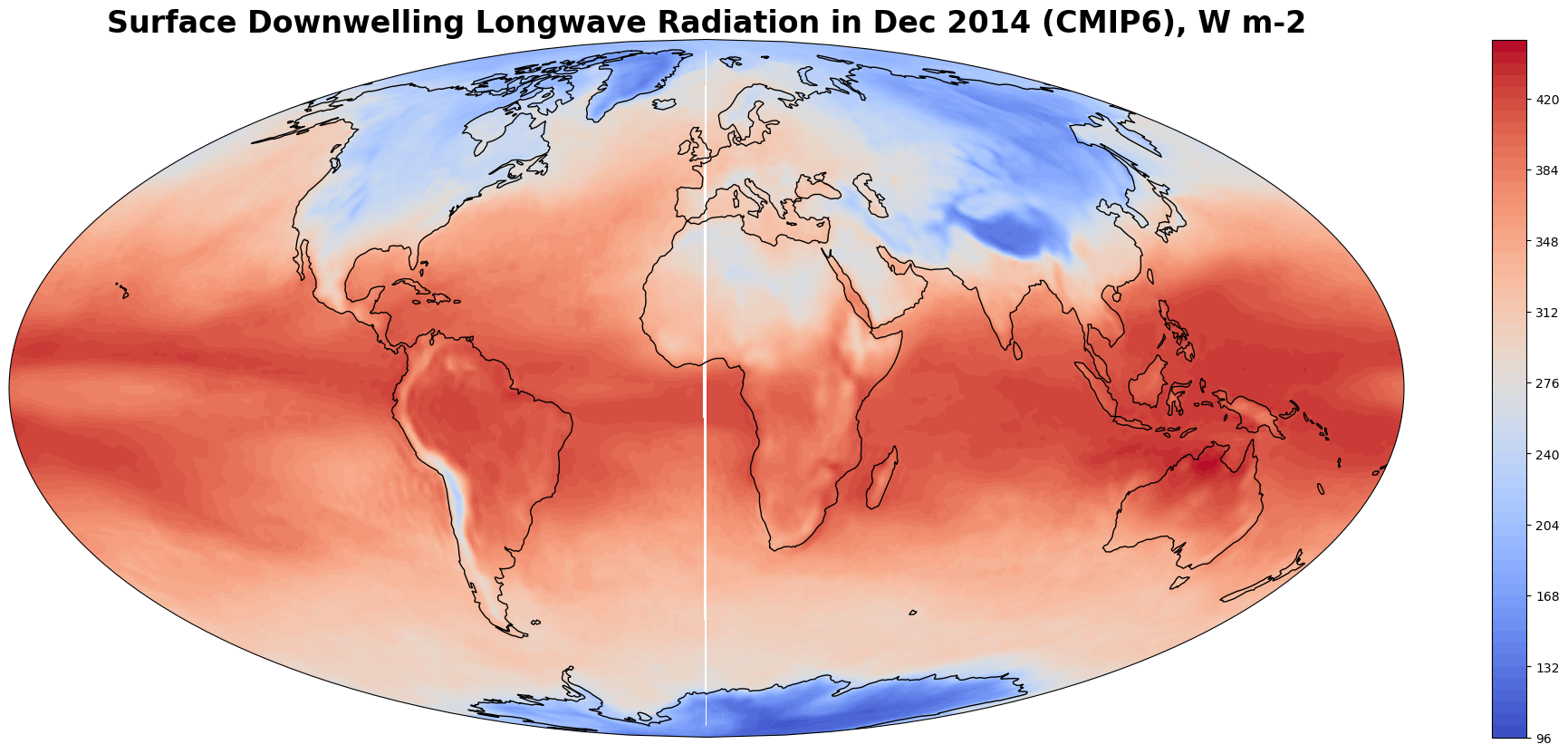
We then load one of the historical monthly CMIP6 models for December 2014 from Mistral, look at its metadata, and plot it.
col = intake.open_esm_datastore("/pool/data/Catalogs/dkrz_cmip6_disk.json")
cat = col.search(variable_id = "rlds",
                 table_id = "Amon",
                 activity_id = "CMIP",
                 experiment_id = "historical",
                source_id = "MPI-ESM1-2-HR",
                member_id = "r1i1p1f1")
xr_dict = cat.to_dataset_dict()
dset = xr_dict[list(xr_dict.keys())[0]]
dset['rlds']
/home/k/k204199/.conda/envs/summerschool_2022/lib/python3.10/site-packages/intake_esm/core.py:84: DtypeWarning: Columns (21,22,23) have mixed types.Specify dtype option on import or set low_memory=False.
  self._df, self.catalog_file = _fetch_catalog(self.esmcol_data, esmcol_obj, csv_kwargs)
--> The keys in the returned dictionary of datasets are constructed as follows:
	'activity_id.source_id.experiment_id.table_id.grid_label'
<xarray.DataArray 'rlds' (member_id: 1, time: 1980, lat: 192, lon: 384)>
dask.array<broadcast_to, shape=(1, 1980, 192, 384), dtype=float32, chunksize=(1, 60, 192, 384), chunktype=numpy.ndarray>
Coordinates:
  * time       (time) datetime64[ns] 1850-01-16T12:00:00 ... 2014-12-16T12:00:00
  * lat        (lat) float64 -89.28 -88.36 -87.42 -86.49 ... 87.42 88.36 89.28
  * lon        (lon) float64 0.0 0.9375 1.875 2.812 ... 356.2 357.2 358.1 359.1
  * member_id  (member_id) <U8 'r1i1p1f1'
Attributes:
    standard_name:  surface_downwelling_longwave_flux_in_air
    long_name:      Surface Downwelling Longwave Radiation
    comment:        The surface called 'surface' means the lower boundary of ...
    units:          W m-2
    original_name:  rlds
    cell_methods:   area: time: mean
    cell_measures:  area: areacella
history: 2019-08-25T06:42:06Z altered by CMOR: replaced missing va...fig = plt.figure(figsize = (25, 10))
ax = fig.add_subplot(1, 1, 1, projection = ccrs.Mollweide())
plt.contourf(dset['rlds'].sel(time = '2014-12-16T12:00:00')[0].lon,
dset['rlds'].sel(time = '2014-12-16T12:00:00')[0].lat,
dset['rlds'].sel(time = '2014-12-16T12:00:00')[0], 60,
transform = ccrs.PlateCarree(0),
cmap = 'coolwarm')
ax.coastlines()
ax.set_global()
# Add a color bar
plt.colorbar(ax = ax)
plt.title('Surface Downwelling Longwave Radiation in Dec 2014 (CMIP6), W m-2',
fontdict = {'fontsize' : '24', 'fontweight' : 'bold'} )
plt.show()

2. Load the observational data#
As an observational dataset we chose the Surface Downwelling Longwave Radiation derived from AHVRR satellite. We download it from the Climate Data Store. https://cds.climate.copernicus.eu/cdsapp#!/dataset/satellite-surface-radiation-budget?tab=form
In sections 2.0 - 2.1 we describe how to retrive the observational dataset from CDS. For the purpose of this workshop, however, we have already prepared this dataset, so you can directly load it in section 2.2.#
2.0 CDS API#
In order to do so we used CDS API which we need to set up first. Please refer to the source git repository for the details on the installation and use of this package. https://github.com/ecmwf/cdsapi
You would need to enter your UID and your API Key to use CDS.
#!pip install cdsapi
# cat > ~/.cdsapirc
# url: https://cds.climate.copernicus.eu/api/v2
# key: <your UID>:<your API Key>
# verify: 0
#pip install cfgrib
import cdsapi
import cfgrib
cds = cdsapi.Client()
2.1 Downlod the data from the CDS#
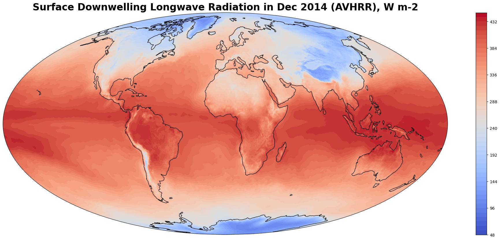
We download the dataset for the same month as our modeling daset, unzip it, load it to the notebook, check its metadata, and finally plot it.
cds.retrieve(
     'satellite-surface-radiation-budget',
     {
         'format': 'tgz',
         'product_family': 'clara',
         'origin': 'eumetsat',
         'variable': 'surface_downwelling_longwave_flux',
         'time_aggregation': 'monthly_mean',
         'climate_data_record_type': 'thematic_climate_data_record',
         'year': '2014',
         'month': '12',
         'version': 'v2_0',
         'sensor_on_satellite': 'avhrr_on_multiple_satellites',
     },
     'download.tar.gz')
/home/k/k204199/.conda/envs/summerschool_2022/lib/python3.10/site-packages/urllib3/connectionpool.py:1045: InsecureRequestWarning: Unverified HTTPS request is being made to host 'cds.climate.copernicus.eu'. Adding certificate verification is strongly advised. See: https://urllib3.readthedocs.io/en/1.26.x/advanced-usage.html#ssl-warnings
  warnings.warn(
2022-08-31 10:01:17,371 INFO Welcome to the CDS
2022-08-31 10:01:17,372 INFO Sending request to https://cds.climate.copernicus.eu/api/v2/resources/satellite-surface-radiation-budget
/home/k/k204199/.conda/envs/summerschool_2022/lib/python3.10/site-packages/urllib3/connectionpool.py:1045: InsecureRequestWarning: Unverified HTTPS request is being made to host 'cds.climate.copernicus.eu'. Adding certificate verification is strongly advised. See: https://urllib3.readthedocs.io/en/1.26.x/advanced-usage.html#ssl-warnings
  warnings.warn(
2022-08-31 10:01:17,478 INFO Request is completed
2022-08-31 10:01:17,479 INFO Downloading https://download-0019.copernicus-climate.eu/cache-compute-0019/cache/data4/dataset-satellite-surface-radiation-budget-d6bfdb4c-680a-48f2-bccb-52052acfe6a5.tar.gz to download.tar.gz (6.3M)
/home/k/k204199/.conda/envs/summerschool_2022/lib/python3.10/site-packages/urllib3/connectionpool.py:1045: InsecureRequestWarning: Unverified HTTPS request is being made to host 'download-0019.copernicus-climate.eu'. Adding certificate verification is strongly advised. See: https://urllib3.readthedocs.io/en/1.26.x/advanced-usage.html#ssl-warnings
  warnings.warn(
0%| | 0.00/6.28M [00:00<?, ?B/s]
3%|███▉ | 191k/6.28M [00:00<00:03, 1.77MB/s]
24%|███████████████████████████████▏ | 1.48M/6.28M [00:00<00:00, 7.80MB/s]
84%|███████████████████████████████████████████████████████████████████████████████████████████████████████████████▍ | 5.30M/6.28M [00:00<00:00, 20.6MB/s]
2022-08-31 10:01:18,048 INFO Download rate 11M/s
Result(content_length=6580570,content_type=application/gzip,location=https://download-0019.copernicus-climate.eu/cache-compute-0019/cache/data4/dataset-satellite-surface-radiation-budget-d6bfdb4c-680a-48f2-bccb-52052acfe6a5.tar.gz)
!tar -xvf download.tar.gz SDLmm20141201000000219AVPOS01GL.nc -C /obs/
SDLmm20141201000000219AVPOS01GL.nc
obs = xr.open_dataset("SDLmm20141201000000219AVPOS01GL.nc").isel(time = 0)
obs
<xarray.Dataset>
Dimensions:    (lon: 1440, lat: 720, nv: 2)
Coordinates:
  * lon        (lon) float64 -179.9 -179.6 -179.4 -179.1 ... 179.4 179.6 179.9
  * lat        (lat) float64 -89.88 -89.62 -89.38 -89.12 ... 89.38 89.62 89.88
    time       datetime64[ns] 2014-12-01
Dimensions without coordinates: nv
Data variables:
    time_bnds  (nv) datetime64[ns] 2014-12-01 2014-12-31T23:59:59
    SDL        (lat, lon) float32 ...
    SDL_nobs   (lat, lon) float64 ...
    SDL_stdv   (lat, lon) float32 ...
Attributes: (12/44)
    title:                           CM SAF Cloud, Albedo and Radiation datas...
    summary:                         This file contains AVHRR-based Thematic ...
    id:                              DOI:10.5676/EUM_SAF_CM/CLARA_AVHRR/V002
    product_class:                   Radiation products, monthly means
    Conventions:                     CF-1.6,ACDD-1.3
    standard_name_vocabulary:        Standard Name Table (v28, 07 January 2015)
    ...                              ...
    cmsaf_parameter_code:            SDL_AVHRR_global_DS
    L3_processor:                    CMSAFGACL3_V2.0, Sirah Software, V1.0
    L2_processors:                   PPS2014 incl. patch 1 and CPP;
    Level1_intercalibration:         1.0
    date_created:                    2016-10-10T08:16:53 UTC
reference_documents: Algorithm Theoretical Baseline Document ...fig = plt.figure(figsize = (25, 10))
ax = fig.add_subplot(1, 1, 1, projection = ccrs.Mollweide())
plt.contourf(obs['SDL'].lon, obs['SDL'].lat, obs['SDL'], 60,
transform = ccrs.PlateCarree(),
cmap = 'coolwarm')
ax.coastlines()
ax.set_global()
# Add a color bar
plt.colorbar(ax = ax)
plt.title('Surface Downwelling Longwave Radiation in Dec 2014 (AVHRR), W m-2',
fontdict = {'fontsize' : '24', 'fontweight' : 'bold'} )
plt.show()

3. Regridding#
As we could find out from the metadata of both datasets, their dimesions are different. We therefore need to regrid one of the datasets before we could spatially overlay them. We will use xESMF and ESMF libraries for this purpose. Please refer to the respective documentation to see the details and parameters of the functions from these packages (https://xesmf.readthedocs.io/en/latest/index.html, https://github.com/esmf-org/esmf).
# In case of problems, activate ESMF verbose mode
ESMF.Manager(debug = True)

# Regridding methods
method_list = ['bilinear','nearest_s2d', 'conservative', 'conservative_normed', 'patch']

# Function to generate the weights
# If grids have problems of degenerated cells near the poles there is the ignore_degenerate option
def regrid(ds_in, ds_out, method, periodic, unmapped_to_nan = True, ignore_degenerate = None):
    """Convenience function for calculating regridding weights"""
    return xe.Regridder(ds_in, ds_out, method, periodic = periodic,
                        unmapped_to_nan = unmapped_to_nan,
                        ignore_degenerate = ignore_degenerate)
Create a regridder for converting the observational dataset to match the model grid.
regridder = regrid(obs, dset, "bilinear", periodic = True, unmapped_to_nan = True, ignore_degenerate = None)
regridder
xESMF Regridder
Regridding algorithm:       bilinear
Weight filename:            bilinear_720x1440_192x384_peri.nc
Reuse pre-computed weights? False
Input grid shape:           (720, 1440)
Output grid shape:          (192, 384)
Periodic in longitude?      True
#Regrid the observational dataset and write write it to the xarray with the modeling dataset.
dset["AVHRR"] = regridder(obs.SDL, keep_attrs = True, skipna = True, na_thres = 1.0)
dset
<xarray.Dataset>
Dimensions:    (time: 1980, bnds: 2, lat: 192, lon: 384, member_id: 1)
Coordinates:
  * time       (time) datetime64[ns] 1850-01-16T12:00:00 ... 2014-12-16T12:00:00
  * lat        (lat) float64 -89.28 -88.36 -87.42 -86.49 ... 87.42 88.36 89.28
  * lon        (lon) float64 0.0 0.9375 1.875 2.812 ... 356.2 357.2 358.1 359.1
  * member_id  (member_id) <U8 'r1i1p1f1'
Dimensions without coordinates: bnds
Data variables:
    time_bnds  (time, bnds) datetime64[ns] dask.array<chunksize=(60, 2), meta=np.ndarray>
    lat_bnds   (lat, bnds) float64 dask.array<chunksize=(192, 2), meta=np.ndarray>
    lon_bnds   (lon, bnds) float64 dask.array<chunksize=(384, 2), meta=np.ndarray>
    rlds       (member_id, time, lat, lon) float32 dask.array<chunksize=(1, 60, 192, 384), meta=np.ndarray>
    AVHRR      (lat, lon) float64 132.0 132.0 132.1 132.1 ... 196.4 196.5 196.5
Attributes: (12/49)
    parent_time_units:       days since 1850-1-1 00:00:00
    parent_variant_label:    r1i1p1f1
    title:                   MPI-ESM1-2-HR output prepared for CMIP6
    nominal_resolution:      100 km
    branch_time_in_parent:   0.0
    cmor_version:            3.5.0
    ...                      ...
    initialization_index:    1
    product:                 model-output
    license:                 CMIP6 model data produced by MPI-M is licensed u...
    further_info_url:        https://furtherinfo.es-doc.org/CMIP6.MPI-M.MPI-E...
    institution_id:          MPI-M
intake_esm_dataset_key: CMIP.MPI-ESM1-2-HR.historical.Amon.gn4. Validate the model#
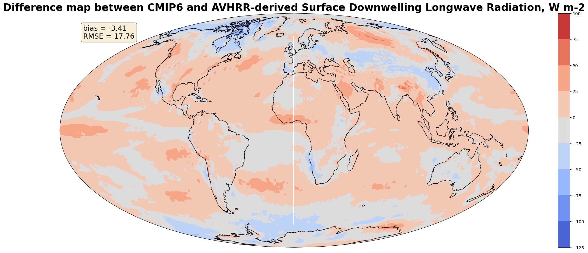
Finally, we can create a difference map between our datasets and calculate its corresponding bias and RMSE.
# Calculate the differene map
diff = dset['AVHRR'] - dset['rlds'].sel(time = '2014-12-16T12:00:00')
diff = diff[:,:,'member_id' == 'r1i1p1f1']

#Calculate the bias and the RMSE
bias = diff.mean().values
rmse = np.sqrt(np.square(diff).sum()/np.square(diff).size).values

# Plot the results
fig = plt.figure(figsize = (25, 10))
ax = fig.add_subplot(1, 1, 1, projection = ccrs.Mollweide())

plt.contourf(diff.lon, diff.lat, diff,
            transform = ccrs.PlateCarree(),
            cmap = 'coolwarm')
ax.coastlines()
ax.set_global()

# Print the bias and the RMSE in a textbox
textstr = '\n'.join((
    r'bias = %.2f' % (bias, ),
    r'RMSE = %.2f' % (rmse, )))

props = dict(boxstyle = 'round', facecolor = 'wheat', alpha = 0.5)
ax.text(0.05, 0.95, textstr, transform = ax.transAxes, fontsize = 17,
        verticalalignment = 'top', bbox = props)

# Add a color bar and a title
plt.colorbar(ax = ax)
plt.title('Difference map between CMIP6 and AVHRR-derived Surface Downwelling Longwave Radiation, W m-2',
          fontdict = {'fontsize' : '24', 'fontweight' : 'bold'} )
plt.show()


